Bayesian Inference

Inference is the process of arriving at generalizations using sample data. Bayesian Inference uses Bayes' Theorem to model the probability of different hypotheses.

$$p(H=h|Y=y) = \frac{p(H=h)p(Y=y|H=h)}{p(Y=y)}$$

• $p(H=h|Y=y)$ is the posterior distribution
• $p(H=h)$ is the prior distribution
• $p(Y=y|H=h)$ is the likelihood, this is not a probability distribution
• $p(Y=y)$ is the marginal likelihood

Bayesian Concept Learning

We can model the distribution of the hidden quantity of interest $h \in H$ from a set of observations, $D = {y_n : n = 1 : N}$, the goal is to infer the hidden patterns or concept from the underlying data.

Humans can generalize a sequence of numbers, based on whether they are all powers of 2, or whether they are even numbers and other similar hypotheses. How do we emulate such process in machines. One classic approach is Induction, here we move from a hypotheses space $H$ of concepts to version space based on the observed data $D$, as more data comes in, we become more certain and the version space shrinks. But the version space theory cannot explain why people choose powers of two when they see $D = \{ 16, 8, 2, 64 \}$ and not all even numbers or powers of 2 except 32. Bayesian Inference can help explain this behavior.

Likelihood

To explain why people go with $h_{two}$ and not $h_{even}$ we will have to understand that it will suspiciously coincidental for all the examples in $D = \{16, 8, 2, 64\}$ to be powers of two if the true underlying hypothesis was $h_{even}$.

Prior

Priori is usefull because, the hypothesis powers of 2 except 32 is more likely than powers of 2, but the former more likely hypothesis is unnatural and we can eliminate such concepts by assigning low priors. Background knowledge or Domain knowledge can be brought into a problem using the prior values.

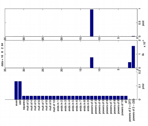
Posterior

Posterior is proportional to likelihood times prior, find below an image that shows how both influence the posterior in identifying the most likely hypothesis for the observed $D$.

Maximum a Posterior (MAP)

MAP is defined as the hypothesis with the maximum posterior probability.

$$h_{map} \triangleq \argmax_h(h|D)$$

Maximum Likelihood Estimate (MLE)

In MAP as the data size increases the prior term stays constant, hence it is reasonable to approximate MAP and just pick maximum likelihood estimate or MLE

$$h_{mle} \triangleq \argmax_{h}p(D|h) = \argmax_{h}\log p(D|h) = \argmax_{h}\sum_{n=1}^{N}\log p(y_n|h)$$

Learning a continuous concept

The game is called healthy levels, we are tasked with identifying the healthy range for two continuous variables cholestrol and insulin from healthy patients, we will be provided with only positive examples. The hypotheses space will be axis parallel rectangles, it can be represented as $h = (l_1, l_2, s_1, s_2)$, where $l_j \in [-\infty, \infty]$ and represents the lower left corner of the rectangle, $s_j \in [0, \infty]$ are the lengths of the two sides.

Likelihood

For 1d we will have $p(D|l,s) = (\frac{1}{s})^N$ if all the points are inside the interval. For 2d we assume the features are conditionally independent given the hypothesis.

$$p(D|h) = p(D_1|l_1,s_1)p(D_2|l_2,s_2)$$

Prior

We will use uninformative priors of the form $p(h) \propto \frac{1}{s_1}\frac{1}{s_2}$.

Posterior

Posterior is given by,

$$p(l_1, l_2, s_1, s_2|D) \propto p(D_1|l_1,s_1)p(D_2|l_2,s_2)\frac{1}{s_1}\frac{1}{s_2}$$

Bayesian Machine Learning

In many applications along with each unknown output $\bold{y}$ we will have features $\bold{x} \in X$ associated with it, in such cases we want to use conditional probability distribution of the form $p(\bold{y}|\bold{x},D)$, where $D = \{(\bold{x}_n,\bold{y}_n) : n = 1:N\}$. If the output is from a low-dimensional space, such as a set of labels $y \in \{1,...,C\}$ or scalars $y \in \mathbb{R}$, then we call it discriminative model, since it discriminates between different possbile outputs. If the output is high dimensional like images or sentences, it is called a conditinal generative model.

In these complex settings, the hypothesis or concept $h$ predictst the output given the input and set of real valued parameters $\theta \in \mathbb{R}^K$.

$$p(\bold{y}|\bold{x},\theta) = p(\bold{y}|f(\bold{x};\theta))$$

Where $f(\bold{x};\theta)$ maps the inputs to the parameters of the output distribution. To fully specify the model, we need to choose the output probability distribution and the form of $f$.

Plugin Approximation

Here we fit a model to compute a point estimate $\hat{\theta}$ and then use it to make predictions. The posterior is represented using Dirac delta function, the point estimates of the posterior are computed using MLE or MAP. The sifting property of the dirac delta helps us arrive at the final form.

$$p(\bold{y}|D) = \int p(\bold{y}|\theta) p(\theta|D) d\theta \approx \int p(\bold{y}|\theta)\delta(\theta - \hat{\theta}) d\theta = p(\bold{y}|\hat{\theta})$$